The Particle Filter

This page is for the reader who wants the machinery. The implementation is clocks.inference.ParticleFilter — a few hundred lines, and everything below maps onto it directly.

State

\(N\) particles, each a full hypothesis for the unknown parameters (e.g. \((x, M)\) in 1D), with weights summing to one. Initialization draws the cloud from the prior — typically uniform over the position and mass ranges.

Update

Per observation, each particle’s log-weight gains the Gaussian log-likelihood of the observed rates given that particle’s predicted rates:

\[\log w_i \mathrel{+}= -\tfrac{1}{2}\sum_c \left(\frac{r_c^{\text{obs}} - r_c^{\text{pred}}(\theta_i)}{\sigma}\right)^2 + \text{const}\]

plus a log-prior that is \(-\infty\) outside the bounds (negative mass, position out of range) — invalid particles die instantly rather than being clamped. Normalization happens in log space (log-sum-exp), because with \(\sigma = 0.005\) the raw likelihoods underflow immediately.

Resampling

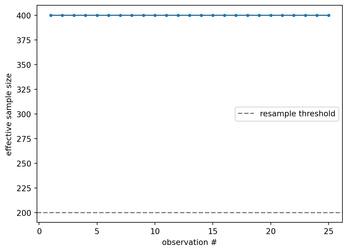
A few sharp observations leave most particles with negligible weight. The effective sample size \(\mathrm{ESS} = 1/\sum_i w_i^2\) measures the collapse; when it drops below resample_threshold · N, the filter redraws \(N\) particles in proportion to weight and perturbs the clones with jitter so they don’t sit on top of each other. Three resampling schemes are available: systematic (the default) walks one evenly-spaced comb with a single random offset through the cumulative weights, giving minimal variance; stratified draws one uniform sample per equal-probability stratum, trading a little variance for independence between strata; residual deterministically copies each particle \(\lfloor N w_i \rfloor\) times and only randomizes the remainder. Two jitter modes:

fixed — isotropic Gaussian noise with absolute scale jitter_std.
covariance — noise shaped by the weighted empirical covariance of the cloud, scaled by jitter_std. When the posterior is a thin diagonal ridge (a “banana”), isotropic jitter pushes particles off the ridge; covariance jitter slides them along it.

The covariance mode has a guard worth knowing about: with fewer than two effective particles the weighted covariance is mathematically undefined (np.cov’s normalization \(1 - \sum w_i^2\) hits zero), so the filter falls back to isotropic jitter for that resample rather than crashing or freezing.

Evidence

Each update’s increment \(\log \sum_i w_i L_i\) is the marginal likelihood of that observation under the model — how well the model predicted the data before seeing it. Summed over observations this is the log-evidence, the quantity model comparison ranks.

Watch the ESS breathe

Code

import matplotlib.pyplot as plt
import numpy as np
from clocks import (
    ClockArray, InferenceConfig, MassConfig, NoiseConfig,
    PriorConfig, SimulationConfig, build_particle_filter, simulate,
)

clock_array = ClockArray(positions=np.array([[-5.0], [0.0], [5.0]]), track_offset=1.0)
truth = MassConfig(positions=np.array([[2.5]]), masses=np.array([0.8]))
sim = simulate(SimulationConfig(
    clock_array=clock_array, ground_truth=truth,
    noise=NoiseConfig(observation_std=0.005), n_observations=25, seed=42,
))
pf = build_particle_filter(InferenceConfig(
    clock_array=clock_array, noise=NoiseConfig(observation_std=0.005),
    prior=PriorConfig(position_range=(-8.0, 8.0), mass_range=(0.1, 2.0)),
    n_particles=400, n_masses=1, seed=42,
))

ess_trace = []
for obs in sim.observations:
    state = pf.update(obs)
    ess_trace.append(1.0 / np.sum(state.weights**2))

fig, ax = plt.subplots()
ax.plot(np.arange(1, 26), ess_trace, marker="o", ms=3)
ax.axhline(0.5 * pf.n_particles, ls="--", color="gray", label="resample threshold")
ax.set_xlabel("observation #")
ax.set_ylabel("effective sample size")
ax.legend()
plt.close(fig)
fig

Effective sample size over 25 observations. Sharp likelihoods crash it; resampling (below the dashed threshold) resets it to N.

Failure modes

Three ways this machinery can lie to you, and what the library does about each:

Weight collapse. Every particle lands at \(-\infty\) log-weight (prior and data contradict). The filter raises RuntimeError instead of propagating NaN.
Particle impoverishment. After resampling, the cloud consists of near-identical clones; if the jitter is too weak the posterior freezes and reports false certainty. This is the failure that motivated the demos shipping with fixed jitter.
Label switching. With multiple masses, the posterior is symmetric under relabeling; the sorting constraint breaks it, at a known cost near the sort boundary.