Into the Plane

Same physics, more geometry

Nothing in the forward model or the filter knows about dimensions. The potential sums \(-M_j/r_{ij}\) over whatever coordinates you hand it; only the prior gains a column when the mass can hide in a plane instead of on a line. The interesting changes are geometric:

  • The eight clocks are scattered asymmetrically across the region. A perfectly symmetric ring would leave mirror-image mass positions indistinguishable; asymmetry is free information.
  • The clocks sit at a perpendicular offset (track_offset=3.0) from the mass plane. Without it, a hypothesis that drifts right on top of a clock could explain that clock’s reading with an arbitrarily small mass — the offset keeps the geometry informative.

The 2D search: 8 clocks, one hidden mass, three unknowns (x, y, M).

The surviving hypotheses

Scaled down and executed on this page, here is what the particle cloud looks like after 25 observations:

Code
import matplotlib.pyplot as plt
import numpy as np
from clocks import (
    ClockArray, InferenceConfig, MassConfig, NoiseConfig,
    PriorConfig, SimulationConfig, infer, simulate,
)

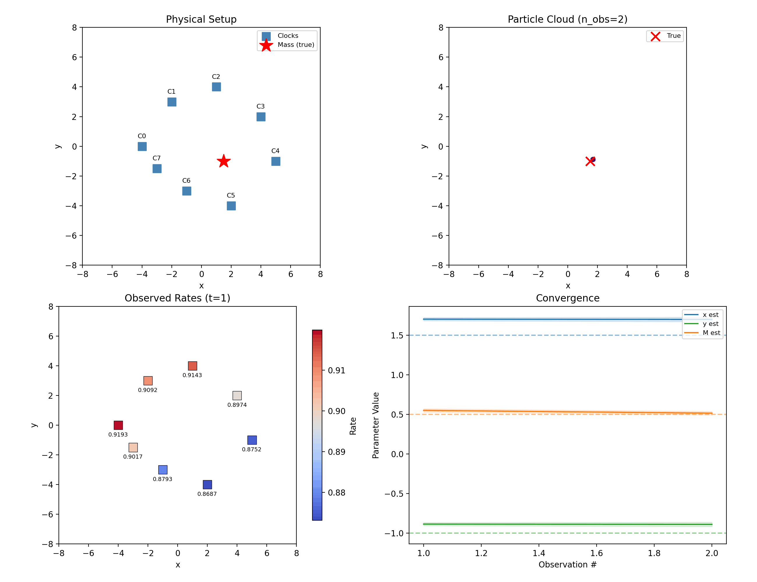
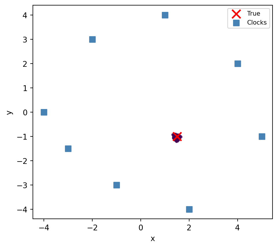
clock_positions = np.array([
    [-4.0, 0.0], [-2.0, 3.0], [1.0, 4.0], [4.0, 2.0],
    [5.0, -1.0], [2.0, -4.0], [-1.0, -3.0], [-3.0, -1.5],
])
clock_array = ClockArray(positions=clock_positions, track_offset=3.0)
truth = MassConfig(positions=np.array([[1.5, -1.0]]), masses=np.array([0.5]))
sim = simulate(SimulationConfig(
    clock_array=clock_array, ground_truth=truth,
    noise=NoiseConfig(observation_std=0.005), n_observations=25, seed=42,
))
result = infer(sim.observations, InferenceConfig(
    clock_array=clock_array, noise=NoiseConfig(observation_std=0.005),
    prior=PriorConfig(position_range=(-8.0, 8.0), mass_range=(0.1, 2.0)),
    n_particles=500, n_masses=1, seed=42,
))

particles = result.particle_state.particles
weights = result.particle_state.weights
fig, ax = plt.subplots()
ax.scatter(particles[:, 0], particles[:, 1], c=weights, cmap="viridis", s=8, alpha=0.7)
ax.scatter(1.5, -1.0, marker="x", s=120, color="red", linewidths=2, label="True")
ax.scatter(
    clock_positions[:, 0], clock_positions[:, 1],
    marker="s", s=60, color="steelblue", label="Clocks",
)
ax.set_xlabel("x")
ax.set_ylabel("y")
ax.set_aspect("equal")
ax.legend(fontsize=8)
plt.close(fig)
fig

The surviving hypotheses after 25 observations, colored by weight. The red × is the true mass position.

The cloud has collapsed from a uniform smear over a 16×16 box to a tight knot at the truth — three parameters recovered from nothing but tick rates.

Note2D costs particles

The same posterior precision needs a larger cloud as the parameter count grows: candidates must cover a volume, not an interval. Three parameters is still cheap. But this is the curse of dimensionality, and the multi-mass pages — six parameters — will feel it properly.