Clocks as Gravimeters

Time runs slower downhill

Everything on this site rests on one weak-field result from general relativity: a clock sitting at Newtonian potential \(\Phi\) (which is negative near a mass) ticks at a rate

\[\frac{d\tau}{dt} = \sqrt{1 + \frac{2\Phi}{c^2}}\]

relative to a clock far from everything. The factor comes straight out of the time–time component of the Schwarzschild metric; we will not derive it here, just use it relentlessly. Deeper in a gravitational well, \(\Phi\) is more negative, the square root is smaller, and the clock ticks slower. No exotic conditions required — it is true of every clock, everywhere, all the time.

This is measured, not theoretical

Two anchors from the real world:

GPS. As the landing page describes, satellite clocks gain about 45 µs/day from sitting higher in Earth’s potential and lose about 7 µs/day to special-relativistic time dilation. The correction is engineered into the system; without it, positioning would fail within hours.
Optical lattice clocks. Modern clocks reach fractional stabilities near \(10^{-18}\) — good enough to resolve the gravitational redshift from a one-centimeter height change. In 2020, Katori’s group operated two transportable lattice clocks at the base and observatory deck of the Tokyo Skytree and read the 450-meter height difference directly from the difference in tick rates. That experiment is chronometric leveling: surveying with clocks.

A sufficiently precise clock, then, is a gravimeter. An array of them is a gravity camera. The rest of this site asks how sharp a picture that camera can take.

The toy model

To experiment freely we drop to simulation units with \(G = c = 1\) (see Units and Scales for what that means physically). The forward model is two lines of physics: a point mass \(M\) at distance \(r\) contributes \(\Phi = -M/r\), and the clock’s rate is \(\sqrt{1 + 2\Phi}\). The library wraps this in clocks.physics.clock_rates.

Code

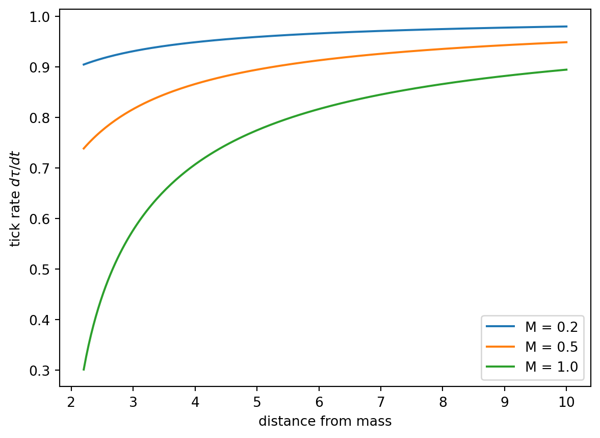
import matplotlib.pyplot as plt
import numpy as np
from clocks import ClockArray, MassConfig, clock_rates

fig, ax = plt.subplots()
# start outside the largest Schwarzschild radius (r_s = 2M = 2.0) so
# rates stay real everywhere on the plot (strong field near the left
# edge, approaching weak field on the right)
distances = np.linspace(2.2, 10, 200)
for mass in (0.2, 0.5, 1.0):
    rates = [
        clock_rates(
            MassConfig(positions=np.array([[0.0]]), masses=np.array([mass])),
            ClockArray(positions=np.array([[d]])),
        )[0]
        for d in distances
    ]
    ax.plot(distances, rates, label=f"M = {mass}")
ax.set_xlabel("distance from mass")
ax.set_ylabel(r"tick rate $d\tau/dt$")
ax.legend()
plt.close(fig)
fig

Tick rate vs distance from a point mass. Heavier masses dig deeper wells; every curve approaches 1 (far-away time) at large distance.

The whole game

That is the whole game: precise timekeeping is gravity sensing. But a camera with one pixel takes a poor picture — and that is exactly the obstacle the next page runs into.