Two Hidden Masses – GPS in Reverse

The problem doubles

Two masses in 1D means four unknowns (\(x_1, x_2, M_1, M_2\)); on a plane, six. The potential is just the sum of the two wells, but the inverse problem gets qualitatively harder, not merely bigger.

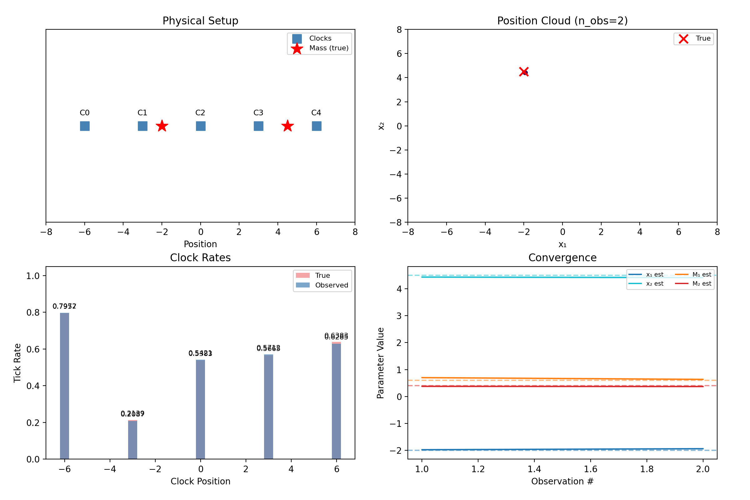
Two masses in 1D: five clocks, four unknowns.

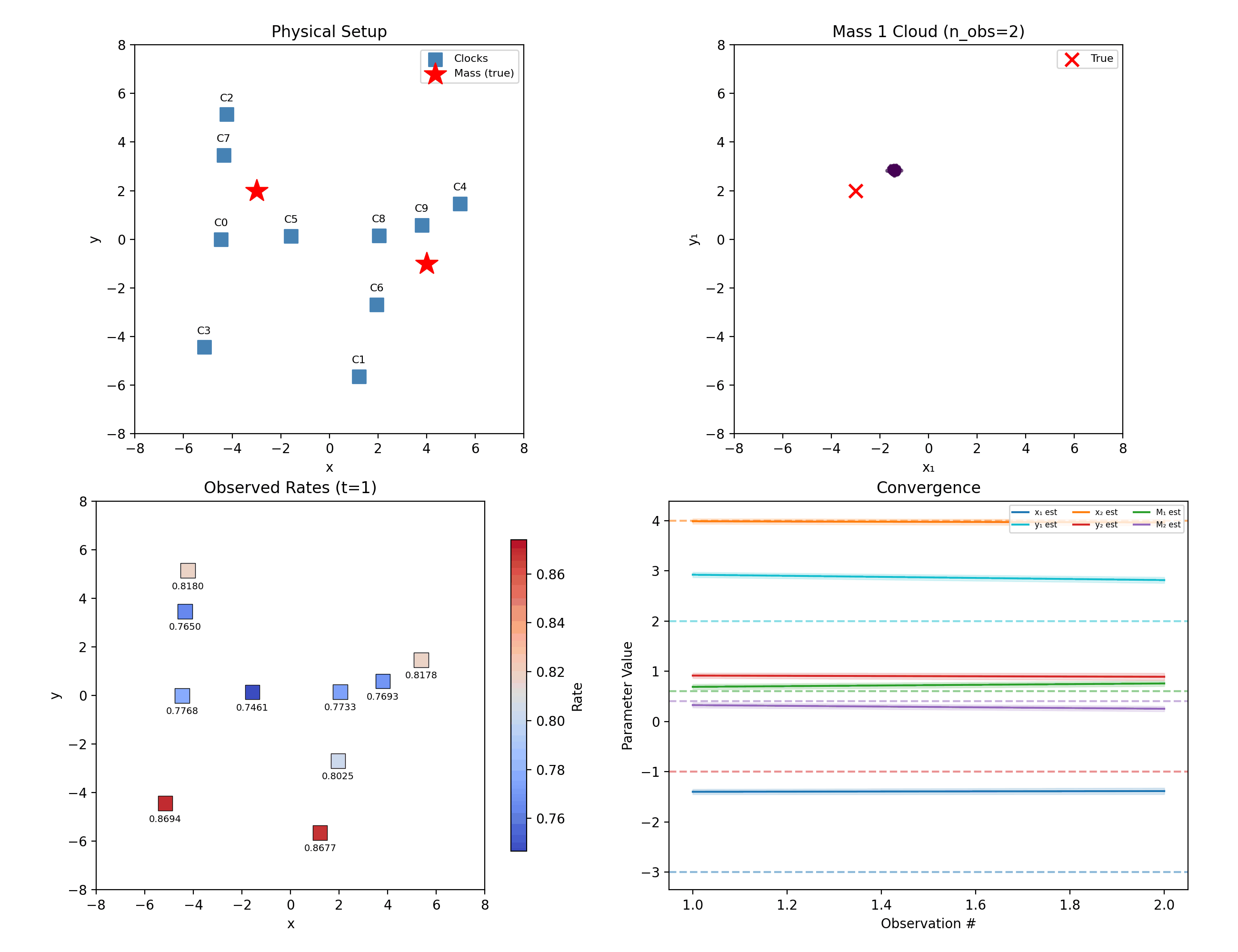
Two masses in 2D: ten randomly placed clocks, six unknowns.

Label switching — an honest limitation

“Mass 1” and “mass 2” are our labels; the physics doesn’t care. A hypothesis with the masses swapped predicts identical clock rates, so the true posterior is perfectly bimodal — and the mean of a bimodal cloud lands meaninglessly between the modes. The library breaks the symmetry by fiat: particles are sorted so \(x_1 < x_2\) at sampling and again after every resampling jitter.

What this does not solve: when the two masses nearly share an x-coordinate, the sort boundary slices right through the posterior, and inference quality degrades. This repo felt that concretely — the 1D demo’s second mass originally sat at \(x_2 = 3.0\), exactly on top of a clock and close enough to cause trouble, and was moved to \(4.5\) to keep the demo crisp. Sorting is a pragmatic fix, not a principled one, and we say so.

Superposition is the enemy

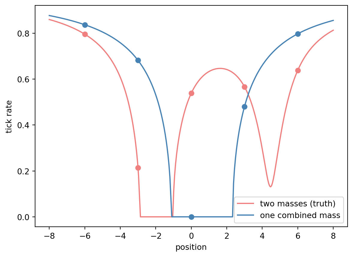
Why is this hard at all? Because summed potentials hide their parts — and the clocks only see the tick rates the summed potential produces:

Code

import matplotlib.pyplot as plt
import numpy as np
from clocks import ClockArray, MassConfig, clock_rates

clock_positions = np.array([[-6.0], [-3.0], [0.0], [3.0], [6.0]])
clock_array = ClockArray(positions=clock_positions, track_offset=1.0)
two_masses = MassConfig(
    positions=np.array([[-2.0], [4.5]]), masses=np.array([0.6, 0.4])
)
one_mass = MassConfig(positions=np.array([[0.6]]), masses=np.array([1.0]))

xs = np.linspace(-8, 8, 300).reshape(-1, 1)
dense = ClockArray(positions=xs, track_offset=1.0)
fig, ax = plt.subplots()
for config, label, color in [
    (two_masses, "two masses (truth)", "lightcoral"),
    (one_mass, "one combined mass", "steelblue"),
]:
    ax.plot(xs[:, 0], clock_rates(config, dense), color=color, label=label)
    ax.plot(
        clock_positions[:, 0], clock_rates(config, clock_array),
        "o", color=color,
    )
ax.set_xlabel("position")
ax.set_ylabel("tick rate")
ax.legend()
plt.close(fig)
fig

Tick-rate profiles for the two demo masses against a single mass of the combined weight placed between them. At the five clock positions (dots), the curves nearly agree — the filter must live off the small residuals.

The filter still separates them — five clocks each contribute a small disagreement, and 80 noisy observations compound those disagreements into certainty. That is the entire trick of the method: no single reading is decisive, and none has to be.

The question behind the question

If two masses can imitate one this well, how would you ever know how many masses are out there? Fixing the number in advance was quietly cheating. The next page stops cheating.