Beyond Point Masses – GPS in Reverse

From particles to fields

Real gravitational anomalies are rarely points — ore bodies, voids, aquifers, anything extended. The same machinery handles them: replace the point-mass forward model with one that integrates the potential over a continuous profile. Here, a Gaussian density with three parameters — center \(\mu\), width \(\sigma\), and peak amplitude \(A\) — and the identical particle filter on top.

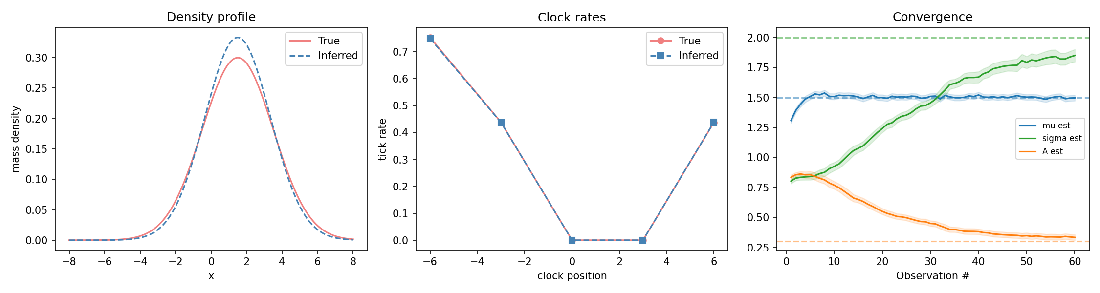
The density demo. Left: true vs inferred density profile. Center: the clock rates both produce. Right: convergence of all three parameters.

What spreading the mass does to clocks

Code

import matplotlib.pyplot as plt
import numpy as np
from clocks import ClockArray, MassConfig, clock_rates, clock_rates_density_gaussian

xs = np.linspace(-8, 8, 200).reshape(-1, 1)
dense = ClockArray(positions=xs, track_offset=1.0)
total_mass = 0.8

fig, ax = plt.subplots()
point = MassConfig(positions=np.array([[1.5]]), masses=np.array([total_mass]))
ax.plot(xs[:, 0], clock_rates(point, dense), label="point mass", color="black")
for sigma, color in [(0.5, "steelblue"), (2.0, "lightcoral")]:
    amplitude = total_mass / (sigma * np.sqrt(2 * np.pi))
    rates = clock_rates_density_gaussian(
        np.array([1.5, sigma, amplitude]), dense
    )
    ax.plot(xs[:, 0], rates, label=f"Gaussian, σ = {sigma}", color=color)
ax.set_xlabel("clock position")
ax.set_ylabel("tick rate")
ax.legend()
plt.close(fig)
fig

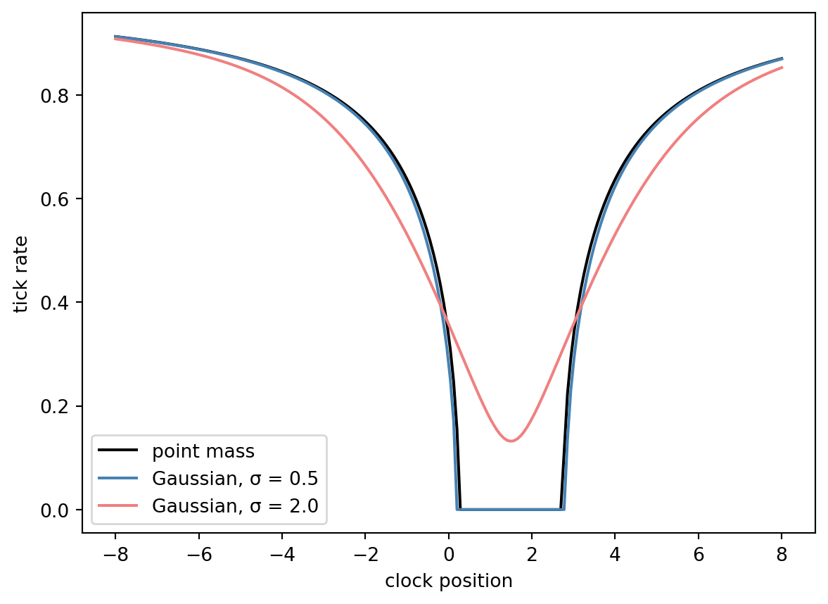
A point mass vs Gaussian profiles of equal total mass at two widths. Spreading the mass flattens and broadens the dip in tick rates.

A new degeneracy

Look back at the demo figure’s left panel: the inferred profile and the true one disagree visibly — yet the center panel shows their clock rates matching almost perfectly. The center \(\mu\) localizes well, but \(\sigma\) and \(A\) trade off along a ridge: a wider, weaker profile and a narrower, denser one can produce nearly identical potentials at a handful of clock positions. This is the mass–distance degeneracy, reborn one level up. The library’s covariance-shaped jitter mode exists for exactly this kind of correlated posterior — it lets the particle cloud slide along the ridge instead of scattering off it.

Where this could go

The repo’s someday-maybe list sketches the next steps: a special-relativity velocity term so SR and GR compete the way they do for real GPS satellites, an MCMC rejuvenation step to make the filter exactly posterior-preserving, and an in-browser interactive version — the inference engine is pure numpy/scipy, which Pyodide already supports.