The Search in One Dimension

The setup

Three clocks sit on a line; somewhere on a parallel track hides a single mass. Two unknowns — position \(x\) and mass \(M\) — and a stream of noisy tick rates. Here is the full search, animated:

The 1D search. Clockwise from top left: the physical setup; the particle cloud in (x, M) space collapsing onto the truth; the convergence of both estimates with uncertainty bands; the observed tick rates being fed to the filter.

Meet the detective

The inference engine is a particle filter: a cloud of hypotheses — one thousand of them in the animation above — each one a guess at \((x, M)\). Every time a new observation arrives, each hypothesis is reweighted by how well it predicts the observed rates; hypotheses that keep predicting badly wither, and resampling multiplies the ones that survive. The cloud is the posterior — its spread is the calibrated uncertainty. Mechanics, knobs, and failure modes live in The Particle Filter.

Watch it converge

The same scenario, run small and live on this page:

import matplotlib.pyplot as plt
import numpy as np
from clocks import (
    ClockArray, InferenceConfig, MassConfig, NoiseConfig,
    PriorConfig, SimulationConfig, infer, simulate,
)

clock_array = ClockArray(positions=np.array([[-5.0], [0.0], [5.0]]), track_offset=1.0)
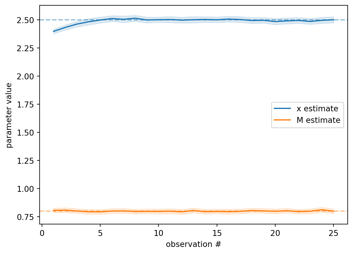
truth = MassConfig(positions=np.array([[2.5]]), masses=np.array([0.8]))
sim = simulate(SimulationConfig(
    clock_array=clock_array, ground_truth=truth,
    noise=NoiseConfig(observation_std=0.005), n_observations=25, seed=42,
))
result = infer(sim.observations, InferenceConfig(
    clock_array=clock_array, noise=NoiseConfig(observation_std=0.005),
    prior=PriorConfig(position_range=(-8.0, 8.0), mass_range=(0.1, 2.0)),
    n_particles=400, n_masses=1, seed=42,
))

steps = np.arange(1, len(result.history) + 1)
means = np.array([entry.mean for entry in result.history])
stds = np.array([entry.std for entry in result.history])
fig, ax = plt.subplots()
for j, (label, true_val, color) in enumerate(
    [("x", 2.5, "tab:blue"), ("M", 0.8, "tab:orange")]
):
    ax.plot(steps, means[:, j], color=color, label=f"{label} estimate")
    ax.fill_between(
        steps, means[:, j] - stds[:, j], means[:, j] + stds[:, j],
        alpha=0.15, color=color,
    )
    ax.axhline(true_val, color=color, ls="--", alpha=0.5)
ax.set_xlabel("observation #")
ax.set_ylabel("parameter value")
ax.legend()
plt.close(fig)
fig

Posterior mean ± one standard deviation per observation. Dashed lines mark the truth: x = 2.5, M = 0.8.

What to notice

The two posteriors do not tighten at the same speed. Position locks in within a handful of observations, because \(x\) is constrained by the ratios between clock readings — geometry that noise mostly cancels out of. Mass rides on the absolute depth of the dip, where every bit of noise counts, so \(M\) keeps a wider band for longer. Asymmetries like this are the filter being honest about which questions the data answers easily — a theme that sharpens when we add a second dimension.