Gravitational Echolocation

A sense you weren’t born with

Imagine someone — call her the synesthete — born with a lattice of atomic clocks embedded in her head — twenty-seven of them, arranged in a neat 3×3×3 grid. Every mass in the world dents spacetime, and clocks deeper in the dent tick slower. Could such a person feel the masses around them, the way echolocation feels surfaces?

One constraint makes this premise honest: the head carries no outside reference. There is no distant master clock to compare against — only the twenty-seven clocks against each other. Whatever is sensed must live in the differences between their tick rates, never in their absolute values.

That is a well-posed physics question, and everything on this site so far — the forward model, the particle filter, the degeneracy analysis — is already dimension-agnostic. So: how far can this sense reach?

What an exterior mass shows the head

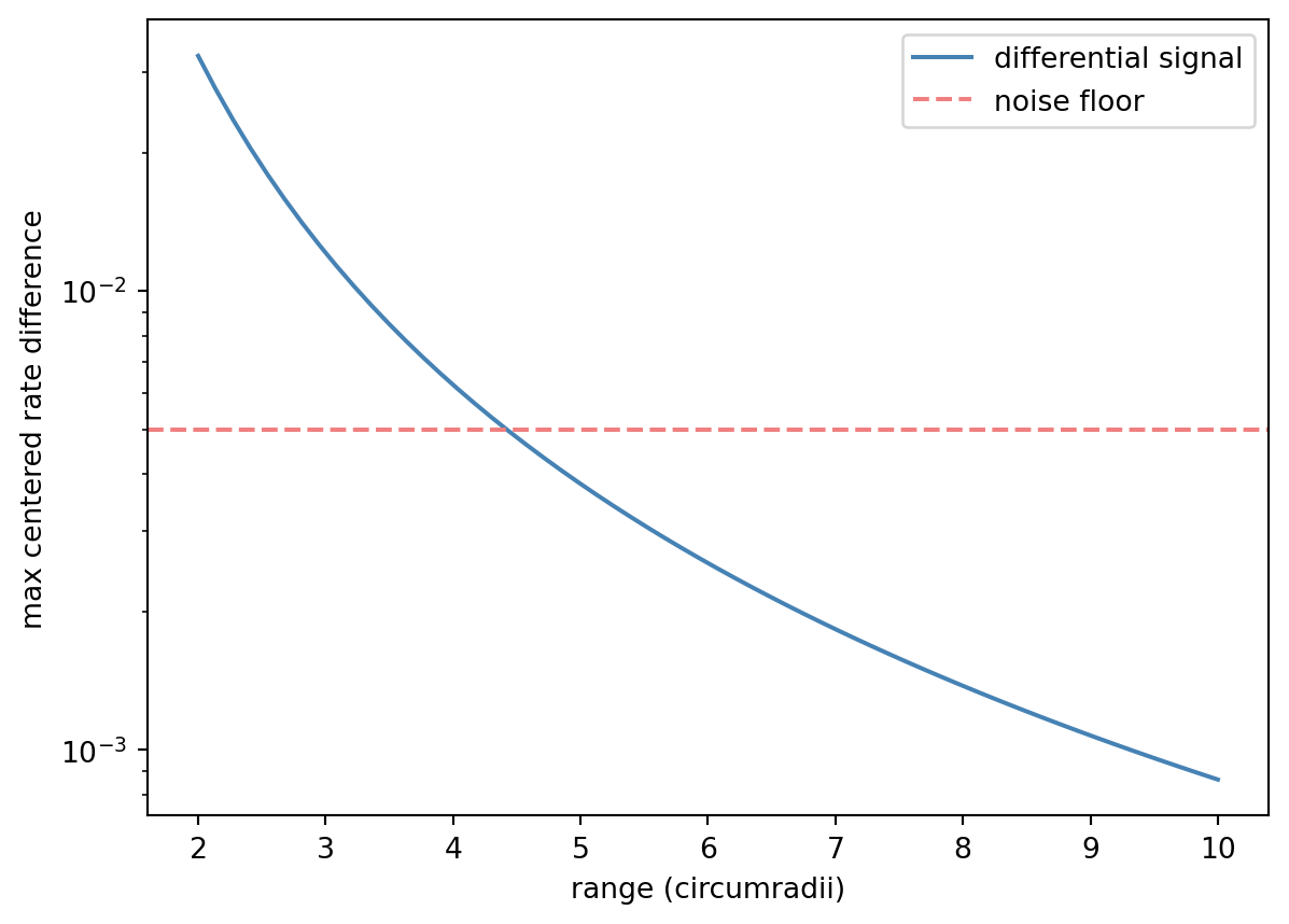
Every previous page hid the mass inside the sensor array. An exterior mass is a harder target: it shifts all twenty-seven clocks by nearly the same amount (a common-mode offset, ∝ M/R), and that shared offset is exactly what the head cannot perceive. Subtract the mean and what remains is the gradient of the potential across the head — falling off as 1/R² — plus the still-fainter curvature that distinguishes “small mass nearby” from “large mass far away.” Direction is cheap; range is expensive. This is the mass–distance degeneracy in its purest form.

import matplotlib.pyplot as plt
import numpy as np
from clocks import clock_rates
from clocks._scenarios import (
    ECHO_NOISE_STD,
    build_head_lattice,
    contrast_matrix,
    echo_mass_config,
)

head = build_head_lattice()
ranges = np.linspace(2.0, 10.0, 60)  # from the validated exterior minimum
signal = []
q = contrast_matrix(len(head.positions))
for r in ranges:
    rates = clock_rates(echo_mass_config(float(r)), head)
    signal.append(np.max(np.abs(q @ rates)))

fig, ax = plt.subplots()
ax.semilogy(ranges, signal, color="steelblue", label="differential signal")
ax.axhline(
    ECHO_NOISE_STD, color="lightcoral", linestyle="--", label="noise floor"
)
ax.set_xlabel("range (circumradii)")
ax.set_ylabel("max orthonormal contrast")
ax.legend()
plt.close(fig)
fig

The differential signal an exterior mass leaves on the head, vs range. The dashed line is the per-observation noise floor; the sense must work in the shrinking gap above it.

The display subtracts the channel mean, but the likelihood uses an exact orthonormal contrast transform. For \(C\) labeled clocks, let \(Q\) have \(C-1\) orthonormal rows perpendicular to the all-ones vector. Then \(Q\mathbf{1}=0\) and \(QQ^T=I_{C-1}\). If the raw channel noise is \(\epsilon\sim\mathcal N(0,\sigma^2 I_C)\), the contrast noise is therefore

\[Q\epsilon\sim\mathcal N(0,\sigma^2 I_{C-1}).\]

The \(C-1\) coordinates preserve the iid variance and the likelihood’s normalization after the unobservable common mode is discarded. Centered \(C\)-vectors remain useful for plotting, but treating their correlated components as independent would give the wrong absolute evidence normalization.

Watching the head lock on

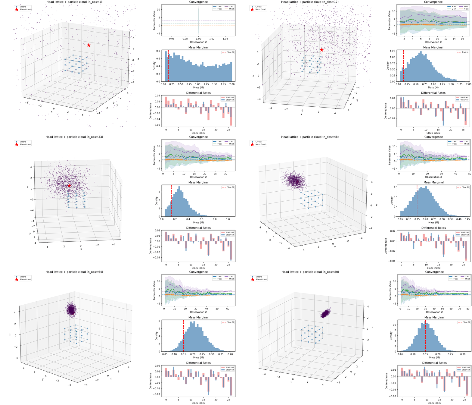
The current default demo places the mass at two circumradii along a fixed off-axis direction and shows eighty differential observations while the camera orbits. It is one fixed-seed visualization at the closest, most favorable range, not a reliability measurement.

The echolocation demo. Left: the head lattice, the true exterior mass (star), and the particle cloud, camera orbiting. Right, top to bottom: parameter convergence, mass marginal, differential rates by clock.

This committed GIF is the current packaged default output from the corrected contrast-space SMC implementation.

How far does the sense reach?

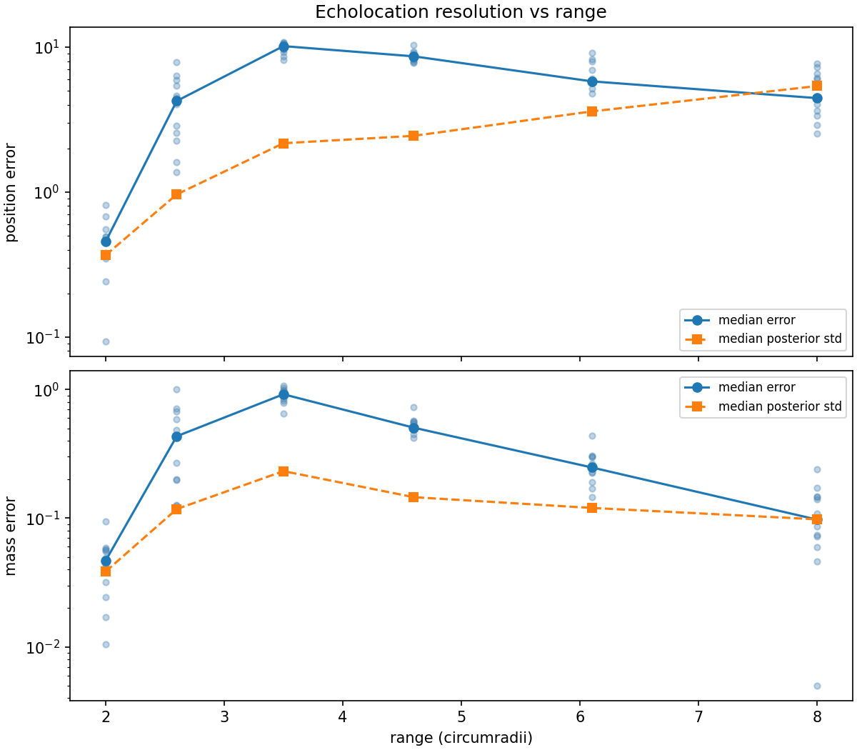
The range harness sweeps the declared circumradius grid and records position error, mass error, posterior standard deviations, coverage, residuals, SMC controls, and forward-model evaluation counts. Development seeds selected and froze the controls and tolerances by the declared ranking. The reserved 400–411 block was then run exactly once for the corrected implementation.

A finite fixed-seed resolution study. Top: position error; bottom: mass error. Dots are individual runs, solid lines are medians, and dashed lines show posterior standard deviations.

The displayed study was regenerated directly from the certified block-400 records. The frozen cell passed 46/72 cases overall; pass counts from close to far were 12, 12, 11, 8, 3, 0. The close range passed 12/12. The far/close median position-standard-deviation ratio was 66.524, above the frozen factor 20 gate, and the 12/12 far-range three-standard-deviation coverage is retained as a diagnostic rather than promoted after inspection into a new gate.

The completed protocol guards against tuning directly to the reported holdout, but its fixed seeds provide regression and calibration evidence only for those simulated cases. It does not estimate population reliability or justify a universal pass probability. The physically robust trend is the signal scaling: the differential gradient falls as \(1/R^2\), while the curvature that helps separate mass from range falls as \(1/R^3\).

Verdict

The surrogate poses a coherent inverse problem inside its \(|2\Phi|\le0.1\) domain, but exterior range is intrinsically difficult. Direction is carried by the leading gradient; separating a nearby small mass from a farther heavy one leans on the weaker curvature. Any claimed sensing horizon must therefore be attached to a stated noise model, prior, particle budget, SMC controls, pass rule, and finite seed set—not promoted to a property of the population.

Coda: could she feel the Sun?

The simulation runs in units where G = c = 1, but nothing stops us from asking the question in SI. Give the head a 10 cm clock baseline. For this estimate, assume a clock budget with fractional-frequency instability near \(10^{-16}/\sqrt{\tau}\) and a systematic floor around \(10^{-18}\) — and ask: sitting long and still enough, could she feel the Sun? Jupiter?

import math

from IPython.display import Markdown

C2 = 8.987551787e16  # c^2, (m/s)^2
BASELINE = 0.1  # clock baseline inside the head, m
SIGMA0 = 1e-16  # clock instability: sigma_y(tau) = SIGMA0 / sqrt(tau)
FLOOR = 1e-18  # systematic floor
GM_SUN, GM_JUP = 1.327124e20, 1.266865e17  # m^3/s^2
AU, R_EARTH, G_SURFACE = 1.495979e11, 6.371e6, 9.80665


def gradient(gm, r):
    """Differential rate across the baseline, held static at range r."""
    return gm * BASELINE / (r**2 * C2)


def tide(gm, r):
    """Surviving differential for a head riding the freely falling Earth.

    Best case: a vertical baseline at the sub-source point, where the
    tidal factor (3 cos^2 theta - 1) reaches its maximum of 2.
    """
    return 2 * gm * R_EARTH * BASELINE / (r**3 * C2)


def sitting_time(signal):
    tau = (SIGMA0 / signal) ** 2
    for label, unit in [("seconds", 1.0), ("hours", 3600.0), ("days", 86400.0)]:
        if tau < 1000 * unit:
            return f"{tau / unit:.0f} {label}"
    years = tau / 3.156e7
    if years < 1e4:
        return f"{years:.0f} years"
    return f"$10^{{{round(math.log10(years))}}}$ years"


def vs_floor(signal):
    ratio = signal / FLOOR
    if ratio >= 1:
        return f"{ratio:.0f}× above"
    ratio = 1.0 / ratio
    if ratio < 1000:
        return f"{ratio:.0f}× below"
    return f"$10^{{{round(math.log10(ratio))}}}$× below"


ROWS = [
    ("Earth, from a chair", G_SURFACE * BASELINE / C2),
    ("Sun, hovering static at 1 AU", gradient(GM_SUN, AU)),
    ("Sun, from a chair on Earth", tide(GM_SUN, AU)),
    ("Jupiter, from a chair on Earth", tide(GM_JUP, 4.2 * AU)),
    ("Jupiter, hovering 100,000 km from center", gradient(GM_JUP, 1.0e8)),
]
lines = [
    "| Source | Differential signal | Sitting time (statistical)"
    " | vs systematic floor |",
    "|---|---|---|---|",
]
for name, s in ROWS:
    lines.append(f"| {name} | {s:.1e} | {sitting_time(s)} | {vs_floor(s)} |")
Markdown("\n".join(lines))

Source	Differential signal	Sitting time (statistical)	vs systematic floor
Earth, from a chair	1.1e-17	84 seconds	11× above
Sun, hovering static at 1 AU	6.6e-21	7 years	152× below
Sun, from a chair on Earth	5.6e-25	\(10^{9}\) years	\(10^{6}\)× below
Jupiter, from a chair on Earth	7.2e-30	\(10^{19}\) years	\(10^{11}\)× below
Jupiter, hovering 100,000 km from center	1.4e-17	50 seconds	14× above

Earth passes immediately. The vertical gradient across her own head is \(1.1\times10^{-17}\). Laboratory clocks have resolved the same gravitational-redshift effect across a single millimeter, about \(1.1\times10^{-19}\) — so a minute or two of stillness gives her down, permanently and unambiguously.

The Sun is stranger. Hovering motionless at 1 AU the signal exists, and seven patient years would statistically resolve it — but it sits two orders of magnitude beneath today’s systematic floor, so that sense waits on the next generation of clocks. And from a chair on Earth the problem changes in kind, not just degree: the Earth free-falls around the Sun, and free fall cancels that leading \(1/R^2\) gradient exactly — the equivalence principle, enforcing itself. What survives inside the head is the tidal residue: real physics, measurable in principle, but four further orders down even with the most favorable alignment, and a million times beneath the floor. No amount of focus recovers the term geometry has removed — no future clock, however good, can measure a signal the equivalence principle has already cancelled. (Earthbound clock networks genuinely do see lunar and solar signatures near the \(10^{-17}\) level — tidal-potential and solid-Earth responses spread across continental baselines. Across a single head, though, that ride is common mode: centering erases it, leaving only the local residue already in the table.)

Jupiter, from Earth, is beyond hopeless. To feel Jupiter she must go there — and hold station, engines burning. Because an orbit is free fall: it removes the leading \(1/R^2\) gradient and leaves only the much smaller tidal residue. Hovering 100,000 km from Jupiter’s center — barely 30,000 km above the cloud tops — Jupiter presses on her clocks as strongly as Earth does from a chair: one meditative minute.

There is a familiar shape in all this. Setting the signal against the \(10^{-18}\) floor gives the head a detection horizon of about 0.08 AU for a Sun-sized mass — and the Sun sits twelve times beyond its own horizon, an illustration of how quickly a differential signal loses to an instrument floor. And even inside the horizon, the caveat becomes absolute at astronomical range: the curvature term that separates mass from distance is suppressed by a further factor of baseline over range, about \(10^{-12}\) at 1 AU. She could feel direction and pull, never distance — a presence, not a place. Which may be the most meditative conclusion physics has on offer.

NoteReproduce

uv run demo-echolocation-3d regenerates the demo; uv run scripts/scan_echolocation_range.py --seed-block 0 --workers 8 --per-run runs the development grid. The reserved run used the scenario-default cell via --seed-block 400; protected blocks reject control overrides. The development defaults and acceptance tolerances were scientifically frozen from seeds 0–11 before the one-shot 400–411 certification. Certification and corrected asset regeneration are complete. See Getting Started.